MRI Physics: Chemical Shift Artifact
Fat and Water
Chemical shift refers to the phenomenon of differing precessional frequencies of protons in fat and water. In fact, protons in different kinds of molecules (and, indeed, different protons within a molecule) resonate at different frequencies in the presence of a magnetic field. This is the basis of NMR spectroscopy (and MR spectroscopy as well). The different frequencies are related to the different electric/magnetic fields these protons experience. Since fat and water are by far the most abundant contributors to the MR signal, these will be our focus. For more discussion of how MR signal is generated and why fat and water are the major contributors, see the section on Tissue Contrast in MRI.
The different local magnetic fields within different molecules mean that protons within those molecules experience different values of B. The frequency difference between protons in fatty acids and water is proportional to the proton Larmor frequency at the given magnetic field and differs by 3.5 parts per million. (Water protons precess slightly faster than fat protons.) In other words, if fH, water at 1.5 T = 63.9 MHz, then γH, fat at 1.5 T = 63.89977 MHz/T. This seems like a very small difference, but it can be relevant depending on our imaging parameters.
Chemical Shift of the "First Kind"
Remember that in MRI, one part of localizing signal to a particular voxel (point in space) is by using frequency encoding. We set up an magnetic field gradient across one axis (e.g. the x-axis), which causes a change in the Larmor frequency at each point since f = γ * B. Now, what happens when fH, water and fH, fat are not the same number? The scanner (well, the Fourier transform) assumes that any signal with a certain frequency came from a certain voxel - so it will make a mistake about where the fat pixels are compared to the water pixels. The scanner places all signals with a certain small range of frequencies into the same pixel 'bin'; this frequency range depends on the bandwidth (described in detail in the MR image formation parameters section). Note that since this phenomenon is caused by frequency shifts, it applies to the frequency-encoding direction only.
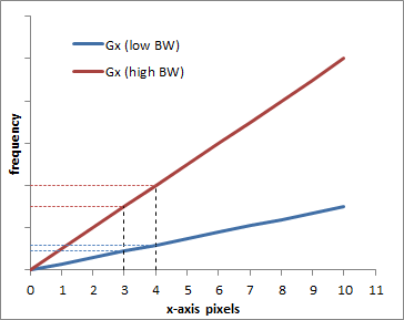
Graph illustrating the difference between a low BW = low gradient (blue) and a high BW = high gradient (red). Obviously, the frequency difference between pixel 0 and pixel 10 is bigger with the higher gradient, which is why a larger bandwidth is needed. The graph also shows how each pixel (e.g. pixels 3 and 4) are more separated in frequency with the higher bandwidth.
You can easily calculate the 'frequency width' of a pixel like so, given the total bandwidth (BW) for the sequence:
Δf / pixel = BW / matrix size
For example, if the BW = 32 kHz and the matrix size is 256, then Δf / pixel, also referred to as BW/pixel, is 125 Hz. Now, as shown above, the frequency difference between fat and water is γH * B0 * 3.5/1,000,000 = 224 Hz at 1.5 T. That means that signal from fat and water is separated by 224 Hz, but pixels are divided at 125 Hz - so the fat and water signal from the same voxel show up in different pixels.
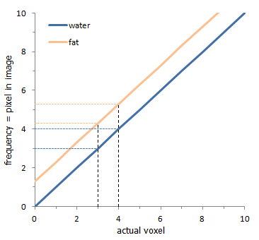
Graph of the chemical shift phenomenon. The x-axis delineates voxels in the tissue, while the y-axis shows the frequency shift generated by the readout gradient and chemical shift. The dashed lines illustrate that the protons in a voxel (here, between 3 and 4) map to different pixels: for fat (orange), they map to pixels 4-5 (and a little 5-6); for water (blue), they map to pixel 3-4.
|
Matrix Size: 256. B0: 1.5 T. Bandwidth:kHz Δfwater-fat: 224 Hz Misregistration: pixels |
Illustration of the chemical shift phenomenon in a simulated image of a kidney. The fat and water signals shift along the frequency-encoding (x) axis depending on the bandwidth, i.e. readout gradient strength. You will observe black and white outlines around the interfaces between organs and fat because signal from some water pixels will be missing from their correct locations, and there will be extra signal from water pixels on the other side.
As you can see from the formula, the chemical shift artifact is worse at higher field strengths. It is not seen on fat-suppressed images, for obvious reasons. It is present on both spin echo and gradient echo images, as opposed to chemical shift of the 'second kind', below.
Chemical Shift of the "Second Kind"
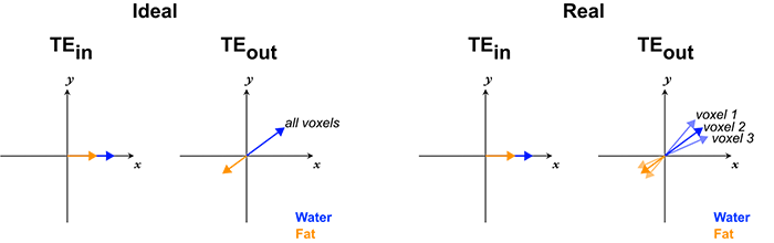
The second manifestation of chemical shift relies on the exact same underlying effect but appears in a different context. Remember again that fat and water protons precess at slightly different frequencies. Similar to playing two tuning forks with slightly different frequencies at the same time, the summed signal contains "beats" - or variations in loudness - at a frequency equal to the difference in the two frequencies. This is the result of the trigonometric identity
sin(f1 * t) + sin(f1 * t) = 2 * sin((f1+f2) * t/2) * cos((f1-f2) * t/2)
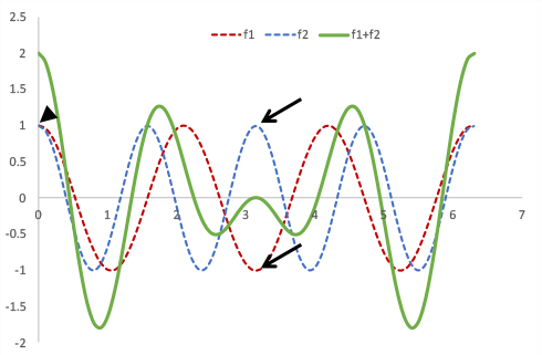
Two signals with different frequencies (red and blue lines) start in phase but cycle in and out of phase (arrows show the point at which they are 180 degrees out of phase). The green line shows their sum, which varies at a different rate. Note that it is zero when the two signals are completely out of phase.
The phenomenon of signal cancellation based on phase differences is often referred to as "destructive interference" (constructive interference refers to the phenomenon of signals adding when they are in phase). Water and fat protons exhibit the same behavior - they go in and out of phase with each other over time, based on the difference in their frequencies (which, as we know, is 3.5 ppm of the Larmor frequency). If we purposefully acquire the signal when they are out of phase, we will get the difference between the fat and water signals (they will cancel each other out, with the more abundant substance left over). If we image them when they are in phase, we will get the sum of their signals. Since the protons start precessing at the 90-degree pulse, this is all dependent on the TE.
In order to find out the correct imaging time for out-of-phase signal, remember that time (period) = 1/frequency. The sinusoid signal for the phase difference has a frequency determined by the water-fat difference in frequencies, so at 1.5 T:
Phase period = 1 / fdifference = 1 / 224 Hz = 4.4 ms
The signals start in phase, get completely out of phase half-way (4.4 ms / 2 = 2.2 ms), then come back into phase at 4.4 ms. The cycle keeps repeating every 4.4 ms (at 1.5 T). Thus,
TEout-of-phase = 2.2 ms and TEin-phase = 4.4 ms
You could also use TEout-of-phase = 6.6 ms and TEin-phase = 8.8 ms, since the cycle repeats every 4.4 ms. At 3 T, we can do the same calculation: Δf = 3.5/1,000,000 * 42.6 MHz/T * 3 T = 447 Hz. The phase difference oscillates at 1 / 447 Hz = 2.2 ms (which is twice as fast as at 1.5 T). Now, in principle that means we can use TEout-of-phase = 1.1 ms. However, it turns out that this is too short for the gradients and MR electronics to perform the actual pulses, so instead we typically use
TEin-phase = 2.2 ms and TEout-of-phase = 3.3 ms
Chemical shift artifact of the second kind does not occur in spin echo sequences. This is because the 180-degree pulse 'rewinds' the phase shifts:
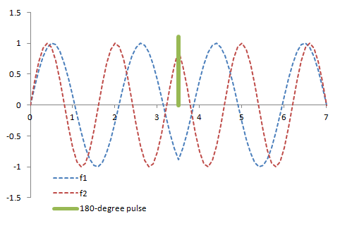
Illustration of the two signals with different frequencies (red and blue lines) in a spin-echo sequence. The 180-degree pulse reverses the direction of the precession so the signals are 'rewound' back to being in phase at the time the echo is sampled.
We can take advantage of the in-phase and out-of-phase effects to look for intra-voxel fat. Any pixel that contains both fat and water should have a lower signal intensity on the out-of-phase images. We often use this clinically to look for hepatic steatosis or intravoxel fat in an adrenal adenoma. Note that pixels that are all fat will not lose their signal in out-of-phase images. Thus, the macroscopic fat in an angiomyolipoma of the kidney, for example, will remain hyperintense.
Dixon Technique of Fat Suppression
We can use the chemical shift (second kind) effect systematically to remove all the fat from an image. As we noted, for the in-phase images, the fat and water signals add, and for the out-of-phase images, the fat and water signals are subtracted. In other words, the intensities I have the following relationships
Iin = Iwater + Ifat, Iout = Iwater - Ifat
which means that
Iin + Iout = 2 * Iwater and Iin - Iout = 2 * Ifat
|
In-Phase Out-Of-Phase Water-Only = In + Out Fat-Only = In - Out |
Simulated Dixon sequence image of a kidney and perirenal fat.
This is referred to as the Dixon method of fat suppression - you simply acquire the in- and out-of-phase echoes and then add and subtract them to create "water-only" (fat-suppressed) and "fat-only" images. As with STIR sequences, this method is relatively resistant to magnetic field inhomogeneities.
Magnetic Field Inhomogeneities. The above discussion is in fact oversimplified to the point of being wrong. Recall that, because of magnetic field inhomogeneities, protons in different parts of the image precess at slightly different frequences. (In fact, this is the phenomenon we employ to our advantage in spatial localization.) For this reason, protons in different parts of the image end up with slightly different phases between the in-phase TE and the out-of-phase TE.
You might think that for the same reason, the time (TE) at which water and fat become 180 degrees out-of-phase will also differ for each voxel in the image. While this is true in principle, the difference is so small to be practically insignificant. You can understand this by realizing that the magnetic field inhomogeneity in the B0 field is quite small (on the order of 1-5 ppm) and the difference in precession frequency between fat and water is also quite small (3.5 ppm), so their product is a very small number (parts per trillion).
The voxel-to-voxel phase differences don't affect how we view the in-phase and out-of-phase images, which are both "magnitude" images (most MR images we view in clinical practice are magnitude images; phase data is important in some sequences, such as phase-contrast MRI and phase-sensitive inversion recovery). However, the phase discrepancies make adding or subtracting the in-phase and out-of-phase images problematic.
As we mentioned, one can simply look at the magnitude (amplitude) of the signal in the two images. This operation, the equivalent of absolute value (|x|), ignores the phase differences, so we obtain:
|Iin| = |Iwater + Ifat| = Iwater + Ifat
|Iout| = |Iwater - Ifat| = either Iwater - Ifat if Iwater > Ifat
or Ifat - Iwater if Ifat > Iwater
Notice that the absolute value (magnitude) operation only tells us the largest component of a voxel. We need some more information to figure out if it's fat or water. There are a number of different techniques to get around this problem, which are beyond the scope of this discussion. Some manufacturers use a multi-point Dixon technique (sampling -180, 0, and 180 degrees phase differences between water and fat), but this still is subject to similar problems. Thus, all Dixon-based fat suppression sequences have to use some algorithm to make an educated guess about water versus fat. Again, how they will do this is far beyond the scope of this discussion, but the general principle is simple: one can assume that nearby voxels will have similar composition. Thus, if you know that one voxel is mostly water, you can assume that the next voxel is mostly water; interfaces are usually obvious because the signal will drop to zero on the out-of-phase image. Usually these algorithms are successful, but they can make mistakes leading to an entirely wrong guess (the "water" image will actually be the fat image) or to parts of an image that are guessed incorrectly as in the example below.
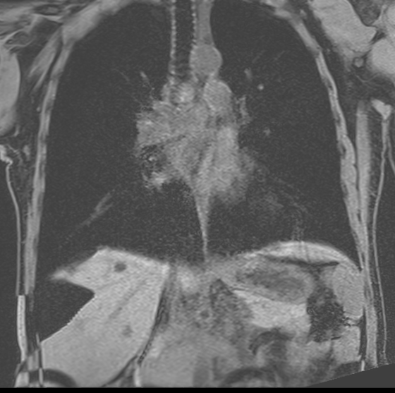
Example of a fat-water swap in a Dixon-based sequence (notice the right hepatic lobe).
Things to Remember
- Fat and water protons precess at slightly different frequencies because of molecular structure. The effect is proportional to field strength.
- This results in a shift in where the scanner thinks the signal is coming from along the frequency-encoding axis. The degree of shift is dependent on the receiver bandwidth (higher BW -> less chemical shift).
- The chemical shift phenomenon can be taken advantage of to obtain in-phase (water+fat) and out-of-phase (water-fat) images in gradient echo sequences.
- By mathematically combining the in-phase and out-of-phase images, you can obtain water-only (fat-suppressed) images, a method known as the Dixon technique.
References
- Hashemi, R. H., Bradley, W. G. & Lisanti, C. J. MRI: the basics. (Lippincott Williams & Wilkins, 2010).
- Hood MN, et al. "Chemical shift: the artifact and clinical tool revisited." Radiographics. 1999 Mar-Apr;19(2):357-71.
- MRI-q.com
- Ma J. "Dixon techniques for water and fat imaging." J Magn Reson Imaging. 2008 Sep;28(3):543-58. Pubmed
Content, including applets and images, copyright 2013-2014 Mark Hammer. All rights reserved.