CT Physics: Dose Measurement in CT

Different Measures of Dose

We need to start by first explaining what dose is, why we care about it, and what different ways there are to measure it. You can read a similar discussion focusing on dose in Radiography in that section. There's also a brief discussion of the effects of Pitch on dose in our section on Helical CT, and we will touch on that later in this page as well.

Dose represents the amount of energy deposited in tissue from radiation per mass of tissue, and is measured in J/kg = Gray (Gy). Note that because it is energy per unit mass, depositing 1 Joule of energy in a 1 kg foot is the same dose as depositing 15 J to the abdomen, which weighs about 15 kg.

What happens when this energy is deposited? Well, obviously it is important for the x-ray beam to be stopped by the tissue so that we can get pictures. Unfortunately, this energy also damages the tissues it hits. There are two types of adverse consequences of radiation: the deterministic and the stochastic effects. Deterministic effects relate to direct killing of cells by radiation and include (at relevant doses) skin erythema, depilation, and ulceration/necrosis. Stochastic effects relate to genetic damage of cells that can lead to cancer down the line. Importantly, deterministic effects relate directly to the amount of radiation a single cell receives; these require a large dose to become apparent. Stochastic effects can occur (randomly) with very small doses, and even one cell can turn cancerous.

Generally speaking, in CT we are mostly interested in the stochastic effects. The deterministic effects require such a large dose of radiation that it is usually not reached in CT studies. (An exception would include the cases of improperly set-up CT brain perfusion studies, which irradiated the same portion of the head to obtain images over time.) For the stochastic effects, we need to know what tissues got radiation and how sensitive each tissue is to radiation. This information is contained in a measure called the effective dose. The units of effective dose are Sieverts (Sv), which is the same unit as Gray but reflects the fact that conversion factors have been used to adjust for the sensitivity of different tissues.

The similar names and units of dose and effective dose may be confusing since in many ways they represent totally different things. A dose of 1 Gy to the head is not the same as 1 Gy to the breast or 1 Gy to the foot - these tissues have vastly different radiation sensitivities. As noted above, that is the purpose of the effective dose measurement - so that a CT (or really, any radiation study) of one body part with 1 Sv dose represents the same risk of stochastic adverse outcomes as that of another body part that receives 1 Sv. Obviously, a 1 Sv scan of the foot must be a much, much higher dose than a 1 Sv scan of the breast.

Measuring Dose in CT

Getting back to dose - energy deposited in a given mass of tissue - we need to figure out how to measure it in CT. Remember that a CT is basically shooting a lot of x-rays at different angles along a length of the body. We cannot simply add up "each x-ray." In order to measure dose in CT, the CT Dose Index (CTDI) was invented. CTDI, often written as CTDI₁₀₀, is the amount of radiation delivered to one slice of the body over a long CT scan.

Why do we have to use an entire CT scan to measure the dose to one slice? Well, many x-rays scatter into the patient's body - so a good amount of dose to one slice is deposited in adjacent slices. Also, remember that the dose is not uniform from the surface to the inside of the body - the superficial tissues absorb more of the dose, and less radiation reaches the center of the body. Because the CT tube circles the body 360 degrees, this is symmetric* all the way around the body. (*Tube current modulation, such as Siemens CAREDose or GE Auto mA change the amount of radiation based on the direction of the tube so that it's not symmetric; this is discussed more below in the dose reduction section.)

How is CTDI measured? A large tube full of water is placed in the CT scanner and scanned. Because the radiation is not uniform from the edge to the center, measuring devices are placed just below the surface and at the center of the tube. (The "100" in CTDI₁₀₀ refers to how long the radiation measurement device is when the CTDI is measured for a given scanner.) The CTDI calculation assumes that the radiation decreases linearly from the outside to the center and is calculated as CTDI = (1/3) * radiation_center + (2/3) * radiation_periphery. It is then divided by the length of the scan to give a CTDI per slice. So CTDI represents the dose to the tissue in that slice; it depends on the size of the body (more on that later), the tube current and kV, and the pitch.

The CTDI we discussed above, CTDI₁₀₀, is also known as CTDI_w where w stands for weighted. In modern helical CT scanners, the scanner does not simply scan one slice after another. Instead, it scans the entire volume in a helical trajectory. Thus, there isn't really a true 'slice', as the z-position of the scanner is different at each angle. As discussed in the section on helical CT, the spacing between successive revolutions of the CT tube represents the pitch of the scan. (Remember, Pitch = Table movement after 360 degree rotation / Collimator width .) The wider the helix, the less dose the patient receives because the same portion of tissue is being irradiated at fewer angles.

We can convert CTDI_w (=CTDI₁₀₀) to helical mode, and this is called the volume CTDI, or CTDI_vol.

CTDI_vol = CTDI_w / Pitch

As expected, the larger the pitch, the lower the dose. Obviously there are disadvantages of high pitch, which are discussed in detail in the Helical CT section. Many institutions and governing bodies use CTDI_vol as a quality-control measure. For example, the American College of Radiology has set 'reference levels' for adult head, adult abdomen, and pediatric abdomen CTs (75 mGy, 25 mGy, and 20 mGy, respectively).

Now that we have a dose for a single slice, how can we take into account radiation exposure for the entire scan? As a reminder, dose (represented here as CTDI_vol) is an average energy deposition per kilogram of tissue. The dose won't change if you decide to include the entire body in your abdomen and pelvis CT. However, there is a measure of total radiation deposition that we can use, and it is the dose-length product or DLP. As the name implies,

DLP = CTDI_vol * scan length

DLP is usually expressed in units of mGy*cm. Just as discussed in the section on fluoroscopy with regards to the dose-area product, the DLP may provide a better measure of the stochastic risk to the patient after a given CT. It represents not only the amount of radiation to a given tissue (dose) but also the amount of tissue exposed. The DLP can be converted to an effective dose for a 70 kg average patient using lookup tables (which were generated from simulation or phantom measurements). As an example, a paper by Huda and colleagues contains some conversion factors. It is important to remember, though, that these conversions are gross approximations and represent values generated by averaging some example scans. They do not take into account the patient's actual anatomy. For example, if the patient has pendulous breasts that are included in an abdomen/pelvis CT, the breast dose (and therefore, the effective dose) will be much different from that of a patient with small breasts entirely outside of the scan region. Additionally, these conversion factors are not accurate for obese or very thin (or pediatric) patients; see below.

Dose and the Bowtie Filter

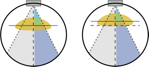
Before we can discuss the effects of patient size on radiation dose in CT, we need to take a small detour to discuss the bowtie filter. If you notice the way an 'ideal' patient or a CT phantom is shaped, i.e. a perfectly round cylinder, you can see that some x-rays from the CT tube pass through very little tissue, i.e. at the periphery, while other x-rays pass through the entire diameter (those through the center of the patient). As you can imagine, this leads to a differential in attenuation between the central rays and the peripheral rays, independent of what the interior anatomy looks like. You can see this in action in the CT simulator.

Why is this a bad thing? Firstly, it is difficult to design detectors for a wide variation in exposure. Secondly, we would like our CT images to appear uniform, and the noise level (which is inversely related to dose) would be lower peripherally and higher in the center. By adding in a filter to decrease the amount of x-rays directed towards the periphery of the patient, we can improve image uniformity and decrease patient dose (by decreasing dose to the superficial parts of the body). This filter is named a bowtie filter after its resemblance to the fashion accessory.

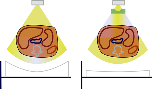
As we noted above, since the bowtie dramatically decreases the dose to the periphery, the CTDI_w (and CTDI_vol) will be decreased. As discussed below, this effect is more pronounced for larger patients. It is important to realize that ideally the bowtie filter should be shaped (or at least sized) to match each patient. Unfortunately, due to design constraints, only a few bowtie filters can be placed in a CT gantry at any one time. Typically, this would include an adult head, adult abdomen, and pediatric; some scanners have cardiac or other specialized bowties. As you can imagine, using filters that do not match the patient's shape will lead to either under-exposing or over-exposing the periphery with respect to the center. Of similar importance is patient centering: if a patient is off-center, the 'center' and 'periphery' won't match up with the bowtie filter.

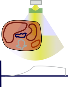
If a patient is not properly centered, increased x-ray flux meant for the center of the patient would fall towards the periphery and over-expose it. At the same time, the center of the patient would now be in the region of decreased x-rays meant for the periphery; this region would be under-exposed and thus appear more noisy in the resulting image. Note that vertical mis-centering will also bias any automated exposure control (tube current modulation) features because it will change the magnification of the scout image; this is discussed further in the dose reduction section.

Patient Size and Dose

As discussed in an earlier section, dose from a CT varies from the surface of the body to the center. As x-rays are attenuated by the surface tissues, fewer reach the center. Since there are fewer x-rays in the center, less dose is deposited there. As noted above, the bowtie filter attempts to make this somewhat more uniform, but there is still less dose at the center. What happens in a fatter patient, assuming the technique is unchanged? Well, (1) their center is farther away from the surface of the patient and so it gets less dose; and (2) their periphery is farther out so it receives less dose because of the bowtie filter. Thus, larger patients receive less dose. Remember that overall, they will receive more total x-rays (even without changing mAs), but dose is per unit mass. It turns out that #1 is only a small effect (dose change of about 10% with a doubling in the diameter of the patient) while #2 represents the majority of the effect with around a 2-fold change in dose for doubling the patient diameter. Smaller patients receive more dose for similar reasons. The calculator below will give you an idea of how patient size affects dose, with data loosely estimated from (Zhou and Boone 2008).

In order to get a proper idea of the dose delivered to a patient, one can use conversion factors for the CTDI known as size-specific dose estimates (SSDE). The conversion of CTDI to SSDE relies on measures of the patient diameter, and the AAPM has published a set of lookup tables. The data in these tables is generated from patient simulation and phantom experiments on various CT scanners and provides a rough estimate of dose. Note, however, that these SSDEs cannot be used to generate effective dose estimates from the lookup tables described above, since obese and skinny patients have different dose distributions and organ distributions. The SSDE can be used to compare dose across obese and skinny patients for technique optimization and quality control.

Dose Reduction Techniques in CT

First, we need to briefly discuss how one can change dose in CT. The major user-accessible parameters are mA, kV, and pitch. We have already discussed pitch. Increasing mA increases the x-ray flux through the patient with consequent increased dose and decreased noise. Increasing kV increases both the x-ray flux and the average x-ray energy with a consequent increase in dose. While noise drops with increased kV, contrast also decreases as the predominating tissue interaction is incoherent scattering rather than the photoelectric effect.

Thus the first - and the traditional - way of adjusting the dose from a CT exam is to simply adjust the mA and kV (and pitch) to the optimal values for that particular examination, with as low dose as possible for acceptable image quality. As mentioned above, the bowtie filter will always be in place and will also provide some dose reduction (and needs to be selected for the relevant body part).

However, it is often difficult to correctly estimate the parameters for a given patient, since these are strongly affected by patient body habitus. Thus, CT manufacturers developed automatic exposure compensation (AEC) methods for CT, which typically involve tube current (mA) modulation. The CT scanner will automatically choose the mA for you based on the scout (topogram) image. The mA will change dynamically along the length of the scan based on the attenuation at that z-position on the topogram.

The importance of the scout scan cannot be underestimated. If the topogram does not include that portion of the scan, the scanner does not know what dose to use and will likely use a default, high dose. Additionally, if the patient is positioned incorrectly in the bore, the topogram might be magnified, and thus the scanner will think the patient is larger than he or she is - and thus deliver a higher dose.

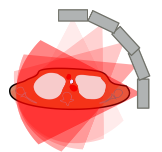
As an additional or alternate method of dynamic mA modulation, many scanners will adjust the mA for the next tube rotation based on how attenuating the tissue was through the last rotation. Separately, most CT scanners will adjust the mA through their rotation angle - depending on how thick the patient is in that direction. In particular, most patients are thicker side-to-side than front-to-back; thus, the scanner will ramp up the mA when the tube is shooting across the patient and decrease it as the tube comes to the vertical angles. Finally, as an even more sophisticated dose-reduction technique, some scanners (e.g. Siemens with CareDose 4D) will reduce the dose across the anterior chest and increase mA through the back of the thorax. This is intended to reduce the breast dose from the scan (but will still obtain diagnostic images since the mA is increased along the equivalent, posterior rays).

How does the AEC decide what mA to use? The fundamental concept is very simple - you want the resulting CT image to look as good in the fat patient as in the skinny patient, right? The scanner will measure the attenuation and size of the patient (at each z-position) based on the topogram and choose an mA to compensate for the size versus the 'standard patient' (and based on the user-entered 'reference' value for image quality). Interestingly, it turns out that radiologists can tolerate noisier images in large patients (perhaps because their body fat provides inherent contrast); thus, some tube current modulation technologies actually increase the mA not quite as much as you would need to give equivalent image quality.

kV and Dose Modulation. The effects of changing kV on patient dose become even more complex in the setting of automated exposure control and with large variations in patient body habitus. CT images can tolerate substantial decreases in kV in small, especially pediatric, patients (e.g. 80 kV), in whom even the lower energy x-rays can penetrate the patient. However, these low energy beams are problematic in very obese patients, in whom they simply cannot penetrate the torso. Thus, the AEC ramps up the mA to compensate. Overall, the exact dose to the patient depends highly on particular scanner settings and should be adjusted to obtain diagnostic images with as low dose as possible.

Things to Remember

• Dose represents the energy deposited per unit mass; in CT, this is represented by the CTDI. Dose depends on mA, kV, and pitch.
• The total energy deposted is the dose-length product. DLP = CTDI * scan length. The DLP can be converted into an estimate of the effective dose, which represents an average risk for stochastic radiation effects (i.e. cancer). However, the CTDI, DLP, and effective dose are not accurate for large or small patients.
• For the same technique, large patients will have lower doses and smaller patients will have higher doses. This illustrates the importance of adjusting the scan settings (mA and kV) for pediatric and obese patients. Automated exposure control (tube current modulation) can perform some of these adjustments for you by using the CT topogram to estimate the patient's attenuation.
• Decreasing the kV can improve contrast and decrease dose, but this is only effective in small and normal-sized patients. Very large patients will attenuate too much of the low-energy x-rays and their doses may actually increase.
• Proper patient centering is critical to avoid excess dose (and noise) from the bowtie filter and AEC system.

References

• McNitt-Gray M. "Assessing Radiation dose – How to do it Right." Talk at 2011 AAPM Dose Summit.
• McCollough C, et al. "Diagnostic Reference Levels From the ACR CT Accreditation Program." J Am Coll Radiol 2011; 8:795. Pubmed.
• Huda W, et al. "Converting Dose-Length Product to Effective Dose at CT." Radiology Sept 2008; 248(3): 995. Pubmed Central.
• Zhou H and Boone JM. "Monte Carlo evaluation of CTDI in infinitely long cylinders of water, polyethylene and PMMA with diameters from 10 mm to 500 mm." Med. Phys. 35(6) June 2008. Pubmed.
• Bushberg JT, et al. The Essential Physics of Medical Imaging. 3rd Edition. Chapter 10. Sec 10.2 describes the bowtie filter.
• Soderberg M and Gunnarsson M. "The effect of different adaptation strengths on image quality and radiation dose using Siemens Care Dose 4D." Radiat Prot Dosimetry (2010) 139 (1-3): 173. Pubmed.
• "Size-Specific Dose Estimates (SSDE) in Pediatric and Adult Body CT Examinations." AAPM Task Group 204. Published 2011. link.

Content and images copyright 2014 Mark Hammer. All rights reserved.