MRI Physics: Diffusion-Weighted Imaging

Diffusion of Water

Molecules in tissue are not fixed in place but move around over time. Some of this motion is related to active processes such as circulation of blood, while other motion is simply random movement with no net goal. This latter phenomenon is related to the heat (energy) in the tissue and is referred to as Brownian motion. As noted, there is no net direction of flow - molecules simply shake and bounce around in solution, moving along a random meandering path, changing direction as they bump into other molecules. The movement of molecules over time is referred to as molecular diffusion.

The motion of these water molecules can be restricted by the presence of barriers, principally cell membranes. You can see an illustration of this process below. The degree of diffusion restriction can be quantified by a diffusion coefficient, which reflects the average distance a particle will move in a second [technically, it is measured in mm²/s because it reflects the area a group of particles will move in a second]; the actual diffusion coefficient is usually not important, but it is useful for terminology.

Free Water	Intracellular Water

Illustration of Brownian motion; left, free water diffusion and right, motion restricted by a cell membrane. Run the simulation several times to see how paths are restricted by the cell. The red line marks the path of the molecule, while the gray line shows the net displacement at the end of the run.

As you might imagine, changes in the cellular density of tissue and the amount of intracellular versus extracellular water will impact the degree of diffusion restriction within that volume of tissue. Conditions such as ischemic infarcts within the brain, pyogenic abscesses, and small round blue cell tumors tend to produce highly restricted diffusion; cysts and edema yield low degrees of diffusion restriction.

Diffusion-Weighted Imaging

Diffusion Gradients. As we have pointed out, diffusion can vary based on an underlying pathology; the ability to measure and compare the diffusion coefficients within an organ is important for a growing number of applications, such as evaluating for acute stroke. An MR pulse sequence can be designed to be sensitive to molecular diffusion, using similar concepts to those responsible for flow-related dephasing and phase-contrast MRA. In particular, particles that move in between the application of two spatial gradient pulses will experience different gradient strengths (since they are in different positions).

Remember that the application of a gradient pulse induces a phase shift in the proton precession; to review this concept, you can read the section on phase-encoding for spatial localization. If we apply a gradient and then reverse it exactly, particles that are in the same location will experience no net phase shift, while particles that have moved will end up with a phase shift.

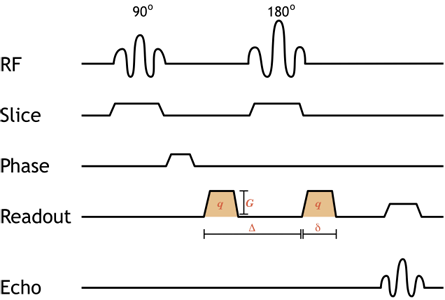
Simplified pulse diagram of a spin-echo diffusion-weighted image sequence. Shaded orange gradients are the diffusion gradients (note that they are both positive since the 180-degree pulse between them reverses the direction of precession, so the second is really negative). The addition of equal, paired diffusion gradients to the standard spin-echo sequence causes moving protons to dephase. The degree of diffusion weighting depends on the strength of the gradient (amplitude G and duration δ) as well as the time spacing between them (Δ) - this is referred to as the b-value, discussed below.

Illustration of the gradients used for diffusion-weighted imaging. In the upper half of the image, two gray stationary protons are depicted; in the bottom half are two blue mobile protons. The diffusion gradient (which varies along the x-axis) is shown at the bottom in red when it is on. The right panel displays the net phase of the 'voxel' containing both protons; the length of the line decreases as the protons dephase. For the stationary protons, note that they are synchronized at the beginning of the pulse sequence, dephase with the gradient, and then rephase as the gradient is reversed. However, the mobile protons cannot rephase since they have moved - they will not experience the same gradient strength as they did initially. These protons accumulate unequal phase shifts, and the net signal is decreased (dephasing).

b value. For a diffusion-weighted image, we can alter the amount of DWI weighting we want, i.e. what our diffusion restriction 'threshold' is. By adjusting the time spacing and strength of the diffusion gradients, we can make the image more or less sensitive to molecular motion. Making the gradient or increasing the time between the dephasing and rephasing gradients will cause much more dephasing from the same amount of Brownian motion. The degree of DWI weighting is referred to as the b-value (quantitatively, b ∝ q² * Δ , where q is the gradient strength and Δ is the time between the two gradients). Low b-value images are only mildly affected by the diffusion properties of tissues. A higher b-value will give a darker image overall, as most tissues will lose signal from molecular motion - but restricted lesions will be more conspicuous; typically we will acquire multiple b values for reasons discussed below to calculate an ADC image. See below for a simulation illustrating this point.

DWI Pulse Sequence. We can now discuss practical details - how does one acquire a diffusion-weighted image? Typical DWI sequences are spin echo sequences, with 90- and 180-degree pulses. (Newer ways of performing DWI are being developed, not all of which use spin echo sequences.) The diffusion gradients are turned on before and after the 180-degree pulse (they are thus both positive gradients because the 180 degree pulse serves to reverse the effect of the second pulse). DWI sequences need to be extremely fast in order to eliminate any motion within the body part - since the entire purpose of the DWI sequence is to measure infinitesimal movements of water molecules, our images will be completely destroyed by macroscopic motions. For a long time, the fastest sequence available was echo-planar imaging (EPI), and virtually all currently used DWI sequences use EPI.

Ideally, we would like our DWI images to be entirely 'DWI-weighted' - in other words, we would only see the results of diffusion, not other properties of the tissue. The TR is long in order to reduce T1 effects and improve signal. The TE is kept as short as possible, but the insertion of the diffusion gradient after the 180 pulse necessitates a longer TE; therefore, DWI images are also T2 weighted. This is a very important point to note - lesions may be bright on DWI from T2 effects alone (this is known as T2 shine-through), and lesions with restricted diffusion and long T2 relaxation will appear very bright!

Fat. Fat creates problems in DWI for several reasons. First, it is bright on DWI images because fat molecules do not move very much (they are relatively restricted); fat signal might obscure lesions. Secondly, chemical shift artifact (of the first kind) is much exaggerated by echo-planar imaging (EPI), often around 10 pixels of a shift! (This is because phase shifts accumulate across the single shot of the EPI sequence; for a techincal discussion, see the references.) Thus, fat from the subcutaneous tissues could obscure lesions in the brain or liver. For both of these reasons, homogeneous fat suppression is necessary for DWI images.

Apparent Diffusion Coefficient

As discussed above, DWI images are inherently T2-weighted. Therefore, lesions with long T2 relaxation will appear bright, even if they do not restrict diffusion. This effect will be particularly apparent on low b-value images, where the diffusion weighting is less (i.e. lesions with fast diffusion have not lost much signal and so will still be bright). Because of its extremely long T2, free water (e.g. CSF, cysts) will be bright even on relatively high b-value images. We would like to eliminate the T2 effects to obtain a more accurate idea of diffusion restriction and eliminate spurious bright spots. In order to do this, we can actually calculate the diffusion coefficient by using several DWI series with different b values.

Apparent Diffusion Coefficient. The diffusion coefficients we measure with MRI represent averages of the entire voxel and of each direction of diffusion (see discussion about anisotropy and DTI later). Therefore, we use the word apparent to describe the values we calculate. The signal of a particular tissue decreases exponentially with increasing b-value. Given an apparent diffusion coefficient D, the signal intensity I is

I = I₀ * e^{-b * D}, where I₀ depends on T2 characteristics

If we acquire at least 2 DWI sequences with different b-values, we can plug them into the equation to solve for D. Typically, at least 3 different b-values are used to improve noise (e.g. 40, 400, and 800); we can take the log of the intensity to linearize the graph and then use linear regression to get a best-fit D. By plotting D for each pixel, we obtain the ADC image (sometimes called an ADC map).

DWI b-value:		ADC

Simulation of how differing b values affect the appearance of DWI images and how to calculate ADC. Left, simulated DWI images showing bright CSF on the low b-value images and increased visibility of the left frontal stroke on the high b-value images. Center, plot of the log of the signal intensity of different tissues (blue, CSF; gray, brain; brown, stroke) at varying b-values. The slope of the line connecting the point is the ADC. Right, simulated ADC image; areas of diffusion restriction, which have the flattest slope on the center plot, have the darkest signal on the ADC image.

Areas of diffusion restriction will lose the least signal on high b-value images (because their protons are not moving). The slope of the line on the DWI plot (see above) will be flat, and thus the ADC value will be small (thus, dark pixels). On the other hand, areas of fast diffusion will lose the most signal as b values increase, giving a large slope - and bright pixels on the ADC image. Importantly, the T2 shine-through - i.e. the brightness on DWI images related to the underlying T2 signal in the tissue only affects the initial position of the points in the DWI plot; it does not affect the slope, thus the ADC image is independent of T2 shine-through - it reflects diffusion alone.

Clinically, we typically still use DWI images because bright abnormalities are much easier to see than dark abnormalities (you may notice this in the simulation above). People have developed several strategies to transform the ADC image into a "bright = bad" map; for example, the exponential ADC (EADC) map takes the exponential of the ADC values, leading to an inverted scale more similar to the DWI (but again, eliminating T2 shine-through effects). Another important reason to use DWI images is that because the ADC image relies on several DWI images, it is inherently more susceptible to artifacts than individual DWI images. Finally, for many abnormalities, they not only restrict diffusion but are bright on T2; thus, we can actually take advantage of the T2 shine-through effect to make lesions more conspicuous, then confirm true diffusion restriction on the ADC map.

Diffusion Tensor Imaging

So far, we have had a simplistic view of diffusion - that water molecules can diffuse in all directions equally. In fact, at least in some tissues, this is not true at all. In highly structured tissues, particularly nerves and white matter tracts in the brain, diffusion happens preferentially along one direction. In white matter, myelin sheaths encircle the neurons and prevent water diffusion across the sheath but allow it along the direction of the axons. Diffusion that is directionally dependent is referred to as anisotropic (i.e. not equal in every direction). That means that if we measure diffusion using gradients in one direction, we would get a different answer than if we measured it in another direction. Equally importantly, if we measure diffusion in one direction, we will get different answers for different parts of the same (healthy) white matter, depending on the direction of the axons in each part.

Intuitively, it would stand to reason that the solution to this problem is to measure diffusion in several directions and create some sort of average - this would cancel out any directional biases. The simplest method to measure the diffusion in different directions is called diffusion tensor imaging or DTI. DTI assumes that within each voxel there is a single directional bias, e.g. a single neuronal bundle direction. It then models the diffusion within an axon not as a scalar (single number) but as a 3-dimensional ellipsoid, which is called a tensor.

Diffusion Tensor

Illustration of the diffusion tensor. A bundle of axons (yellow) is illustrated in 3 dimensions. Water molecules can diffuse along the axons but not across them. The diffusion tensor (brown) represents the diffusion as an ellipsoid, oriented along the axons with the thickness of the ellipsoid in any direction corresponding to the diffusion coefficient in that particular direction. Thus, the ellipse has a thin waist since the ADC is low across axons, but the ellipse is elongated since the ADC is high along the axis of the axons.

From the illustration above, you can see that specifying the diffusion tensor requires two separate sets of parameters: the direction of fastest diffusion (i.e. the direction of the axon bundle) and the actual diffusion coefficients along and across the axons. A direction in 3-dimensional space requires 3 numbers; and the thickness of the ellipse requires 3 numbers (for each axis of the ellipse itself). This means that DTI requires measuring diffusion in 6 different directions. (These directions need to be measured for each non-zero b-value.)

DTI sequences are necessary to produce even regular diffusion-weighted images in the brain - otherwise white matter tracts will look like they restrict diffusion. The mean diffusion images are then produced by averaging three of the directions, and this is what is typically used for DWI and ADC maps. However, by acquiring the 6 different directions, we can also calculate other maps. One of the most common is the fractional anisotropy (FA) map. Recall that anisotropy represents the degree to which diffusion is not the same in all directions; FA is calculated by comparing the lengths of each axis of the tensor ellipsoid to their average. If there is a big difference (such as in the illustration above), then the FA is high, representing anisotropic diffusion. Normal white matter tracts have high FA, which is lost in many disease processes.

Tractography. Finally, DTI can produce good low-resolution images of general white matter tract directions; by calculating the principal direction of the tensor ellipsoid, we get the average direction of axonal bundles in the voxel. We can color code voxels by direction, obtaining a tractography map. Much more sophisticated, high resolution tractography can be obtained by measuring diffusion in more directions. This can take into account areas of crossing fiber bundles (which would just be averaged out in regular DTI). By obtaining these maps, we can create 3-dimensioal in vivo brain connectivity maps. This is currently an area of active research.

Intravoxel Incoherent Motion

Traditional DWI assumes that all water molecules within a voxel behave the same (hence a single ADC per voxel). Of course, this is not true: water molecules experience vastly different environments even within a single voxel. Molecules in flowing blood have a baseline velocity and so diffuse very quickly; intra- and extracellular compartments also have different diffusivity. While the simplistic model is sufficient for most clinical purposes (e.g. stroke), emerging data suggests that some clinically relevant findings may be found in more complex models. The two main categories of advanced diffusion modeling are diffusion kurtosis imaging, not discussed here, and intravoxel incoherent motion (IVIM).

In our above discussion on ADC, we assumed that the relationship between b-value and signal intensity is linear - in other words that there is a single ADC value for a voxel. In fact, in some tissues the relationship is not linear. In particular, the signal intensity drop-off is much steeper at low b values; this implies that there is a small sub-population of very fast diffusing water molecules. This phenomenon is most noticeable in the liver, and it is believed to be related to blood flow in capillaries (though our understanding is incomplete). In order to measure IVIM, instead of measuring ADC using 3 b-values, we need to use more (e.g. 8) - especially at low b-values. Currently, IVIM is being explored as a measure for hepatic fibrosis.

References

Hagmann P, et al. "Understanding Diffusion MR Imaging Techniques: From Scalar Diffusion-weighted Imaging to Diffusion Tensor Imaging and Beyond." Radiographics 26(S1): S205.
Koh D, et al. "Intravoxel Incoherent Motion in Body Diffusion-Weighted MRI: Reality and Challenges." Am J Roentgenol 188(6): 1622.
Dietrich O, et al. "Technical aspects of MR diffusion imaging of the body." Eur J Radiol 76: 314.
"Chemical Shift: Phase Effects." MRI-Questions - discussion about exaggeration of chemical shift in EPI sequences
If you are interested in the original (highly technical!) paper on DWI: Stejskal EO and Tanner JE. "Spin Diffusion Measurements: Spin Echoes in the Presence of a Time Dependent Field Gradient." J Chem Phys 42 (288): 288.