MRI Physics: Pulse Sequences
This page discusses MRI pulse sequences. You may also wish to read about Tissue Contrast in MRI to learn about T1 and T2 properties of tissue or Spacial Localization in MRI to learn about how gradients allow us to image three-dimensional objects. Below is a simulation that incorporates spin echo (SE) and gradient echo (GRE) pulse sequences. Continue reading below to find out how they work.
| T2* effect T2 dephasing Spin Echo Gradient Echo |
|
|
Proton Precession
In MRI, we are imaging properties of hydrogen nuclei (protons) in tissue. Without getting into the details of quantum mechanics, protons behave like tiny magnets; they will tend to line up in the same direction as any external magnetic field. Thus, the first step in MRI is to set up a strong magnetic field (called B0) along the axis of the scanner. The tendency to align along the magnetic field is relatively weak, so random vibrations and collisions of protons within tissue will keep most of them from actually lining up with B0. As an analogy, think of a game of bumper cars with a twist - all of the drivers are trying to point their cars north; because of the crowded field, collisions with other drivers will bump their cars around and keep them from pointing directly north. However, on average, if we look at the whole field, the cars will all be pointing in a northerly direction. In the case of the protons, the bulk magnetization of the tissue - the sum of all of the millions and millions of protons - points exactly along B0.
In addition to trying to align along B0, protons tend to spin or 'wobble' around B0 like a spinning top, a phenomenon termed precession. The speed (frequency) at which they precess is the Larmor frequency, which is determined by a constant (gyromagnetic ratio, γ) times the strength of B0: frequency ω = γ * B0.
Left: Illustration of a proton precessing in a magnetic field (along the green vertical axis). Note that the proton spins around its own axis (large arrow) as well as precessing around the magnetic field. Right: Simulation of many protons precessing in a block of tissue, with B0 pointing up. Note that while each proton is aligned in a random direction, the bulk magnetization (green) points along B0. (Because we are only looking at a small number of protons, the bulk magnetization is not exactly along B0, and you can see it precessing slightly.)
To reemphasize, within a block of tissue, the millions of protons will be precessing in a disorganized fashion and point in different directions - in other words, they are not synchronized. The MRI scanner detects the sum total of these protons: the different directions of wobbling will cancel out, and all that will be left is a slight magnetization pointing along B0 with no wobbling.
One small note: The time it takes for protons within tissue to align with the B0 magnetic field (as best as they will given collisions, vibration, etc.) is related to the T1 of the tissue. After several T1s, the tissue will reach equilibrium. We can the perturb it with excitations - see below - and actually do some MRI!
Proton Excitation
With the protons precessing around B0, nothing interesting will happen and we cannot measure any signal. In order to measure parameters of the tissue, we need to perturb - excite - the system. This is done by applying a transient magnetic field - a radiofrequency pulse - in a different direction from B0; the direction of this pulse is often referred to as B1. Recall that in the presence of a magnetic field, protons will precess around that field. By applying this field for a short time, we can rotate the magnetization of the tissue. If the protons are initially aligned along the z (vertical) axis, and we apply a pulse along the x axis for the right amount of time, we can rotate the magnetization from the z-axis onto the y-axis. This is referred to as a 90-degree pulse, since the magnetization direction is turned by 90 degrees. Once the pulse is turned off, the protons will resume precessing along B0 and will slowly return to their initial equilibrium with the net magnetization pointing along the z axis.
As briefly mentioned earlier, the amount of time it takes for protons to return to being aligned with B0 is determined by the T1 of the tissue. You can find a more detailed discussion of what determines T1 in the page on T1 contrast. While the magnetization is slowly coming up, another process is happening: the magnetization will precess around B0. The net result is a spiral path in the xy plane, as shown below. In MRI, we split the magnetization into two components: longitudinal, along B0 (vertical axis here), and transverse, in the xy-plane. This terminology lets us discuss the two separately; as we have already discussed, recovery of longitudinal magnetization back to its equilibrium is related to the T1 of the tissue.
Illustration of tissue magnetization after a 90-degree pulse. The pulse flips (rotates) the magnetization (green) from the z-axis to the y-axis. The magnetization then precesses, or spins, around B0 as it recovers to its initial state.
Recovery of longitudinal magnetization (i.e. along B0) is an exponential process, and the mathematical formula for magnetization recovery, related to the T1 of the tissue, is:
Mz = 1 - e-t/T1
In the above discussion, we neglected to talk about T2* effects. It turns out that the transverse magnetization disappears much faster than you would expect simply from reorientation towards B0. Recall that the precession speed is determined by the gyromagnetic ratio and the magnetic field strength. Within tissue, each proton experiences a slightly different magnetic field strength - this is related to (a) macroscopic differences in the magnetic field, such as nearby iron or gas and (b) electromagnetic fields produced by the molecules themselves. Because of these differences, the protons even within a uniform tissue will precess at very slightly different rates. The net result of this is that they get out of sync with each other, which is called dephasing.
Illustration of proton dephasing from T2* effects. We are looking down on a set of protons precessing in the xy-plane after a 90-degree pulse. As the protons get out of sync with each other from local magnetic field inhomogeneity, the total tissue magnetization (orange), which is the sum of all protons, drops rapidly.
The speed of dephasing is referred to as the T2* constant; you can read more about what determines T2 of different tissues in the section on tissue contrast in MRI. As the protons dephase, the tissue magnetization drops off rapidly in size. The spinning transverse magnetization is what the MRI scanner can detect with its radiofrequency coils. Thus, signal drops off quickly as the protons precess in the xy-plane, with a speed determined by the T2* value of that voxel.
T2* decay is also an exponential process, like T1 recovery, but it is an exponential decay instead of recovery. The formula is:
Mxy = M0 * e-t/T2, where M0 is the initial magnetization flipped into the xy plane.
In summary, after a 90-degree pulse, the tissue magnetization is rotated so that all of it lies in the xy-plane. This transverse magnetization is what the MRI scanner detects. The magnetization then begins to precess around B0, rapidly losing its size. Somewhat more slowly, the protons realign with B0 and recover their longitudinal magnetization and eventually return to the equilibrium, with the magnetization vector pointed directly along B0. This entire process is often referred to as free induction decay (FID).
T2 and T2*. Dephasing of the transverse magnetization can be split into two types of effects. One type is fixed macroscopic differences in the magnetic field, related to the presence of tissue within the magnet and particular substances such as iron or gas (see further discussion under T2 Contrast). This type of effect does not depend on the contents of the tissue as much as its neighbors - thus, it will be different for muscle next to the lung versus muscle next to the liver. The second type is related to intra- and intermolecular differences in the magnetic field; these differences are rapidly changing as molecules move and vibrate within tissue. However, this type of dephasing depends upon the intrinsic tissue itself and not on its neighbors; it represents the T2 value of the tissue, and you can read more about it in the section on T2 Contrast. The combination of both intrinsic and extrinsic effects is referred to as T2* (T2 star). The distinction between T2* and T2 is important as we discuss the differences between Spin Echo and Gradient Echo sequences.
Spin Echo
As we mentioned, the MR scanner can only detect signal (magnetization) in the transverse plane. We discussed a way to produce transverse magnetization, the 90-degree pulse, above. This produced a free induction decay signal, with the signal decreasing according to T2* effects. There are two disadvantages of this approach: (1) The signal decays very rapidly, requiring an extremely fast scanner to detect it before it dies out; and (2) The signal depends on T2*, not T2, so it is very susceptible to local magnetic field inhomogeneity. In order to combat both of these challenges, we can add another pulse to generate an "echo" that occurs later in time and happens to reverse the T2* effects to leave us with T2 only. This is referred to as the spin echo.
Fixed magnetic field inhomogeneities do not change over time. They lead to fixed differences in proton precession speed across the tissue. The clever solution (discovered by Dr. Erwin Hahn) is to 'reverse' the proton precession so that the faster and slower precessing protons refocus. The often cited analogy is the tortoise and hare race. Imagine the tortoise and hare starting on a race; the hare gets much farther. Then, at a certain time, we tell them both to turn around and come back. They will reach the starting line at the same time - remember that even though the hare is farther out, it is that much faster. In reality, instead of reversing the direction of precession, we rotate the protons with a 180-degree pulse; they continue precessing in the same direction but will refocus along the -y axis, as shown below.
Illustration of the spin echo. Magnetization (green arrows) has been flipped into the transverse plane. It begins to precess, and we see the divergence among 7 protons precessing at slightly different frequencies. At the mid-point of the sequence, a radiofrequency pulse is applied to cause a 180-degree flip in the protons. They continue to precess, with the faster protons reaching the center at the same time as the slower protons.
Notice that the echo, i.e. when the protons precess back to the same point, occurs after the same amount of time has elapsed as before the 180-degree pulse. The time the echo occurs, which is when the MRI scanner acquires the signal, is referred to as the echo time or TE. Thus, the 180-degree pulse must happen at TE/2.
Repetition. As we have discussed, the spin echo sequence has 3 main phases: (1) 90-degree pulse followed by free induction decay; (2) 180-degree pulse followed by rephasing; and (3) the echo that occurs at TE, when the scanner acquires the signal (referred to as readout). We need to repeat this sequence a number of times to acquire the entire image, as discussed in detail in the section on Spatial Localization in MRI. The time between each repetition of the sequence is referred to as the repetition time or TR. We need to wait this time in order to allow the longitudinal magnetization to recover, since that is what we use to generate the transverse magnetization (by the 90-degree pulse) in the next repetition. Changing the TR affects the T1 contrast. We can draw a diagram of the pulse sequence:

Simplified pulse diagram of the spin echo sequence. The top line shows the radiofrequency pulses sent from the scanner, while the middle line shows the MR signal. Note the free induction decay right after the 90-degree pulse and the spin echo at time TE.
We can now add the spatial localization gradients to our discussion and diagram. The slice-select gradient determines which protons get excited - therefore, we need to turn it on during any excitation pulse, i.e. the 90- and 180-degree pulses. Phase-encoding gradients are turned on transiently before readout, to generate the phase shifts; a repetition of the pulse sequence is done for each phase-encoding gradient strength. Finally, the frequency-encoding gradients need to be on during readout, since we need the precession frequencies to be altered while we are measuring them. Thus, the real pulse sequence looks more like this:

Pulse diagram of the spin echo sequence, now including the spatial localization gradients. Remember that each of these gradients is applied in a different direction (e.g. x, y, and z axes). The slice-select gradient is on during excitations, and the frequency-encoding gradient is on during readout (the spin echo).
Fast Spin Echo
The spin echo sequence works very well to generate images with good signal-to-noise. However, it is slow - each phase-encoding step takes one TR. Typical MR images have at least 256 phase-encoding steps, and a typical TR for a T2-weighted sequence is 2-3 seconds: thus, the entire image will take around 600 seconds or 10 minutes! The good news is that we can use the 'dead time' after the echo and before TR to excite another slice in the body and aquire a phase-encoding step in that slice. This means that we can potentially acquire all or many of the slices we need for the body part at the same time. Still, a single sequence will take 10 minutes, a long time to ask a person to hold completely still (and obviously far too long for anything that requires breath-holding). Various techniques can be applied to shorten this time by reducing the number of phase-encoding steps we need, which you can read about in the section on MRI Image Formation Parameters. Here we will discuss a way to modify the pulse sequence to get the same number of phase-encoding steps much faster - the fast spin echo sequence (FSE; sometimes called turbo spin echo or TSE).
Remember that the spin echo occurs after proton dephasing is rephased by the 180-degree pulse. (Again, this only affects fixed magnetic field inhomogeneities; intrinsic T2 dephasing continues unabated.) After the protons become in phase at TE, they will continue to dephase and the 'echo' dies out - but there is nothing stopping us from then sending another 180-degree pulse to rephase them again. We can repeat this 180-degree pulse as many times as we want, each time generating an echo from negating the effects of fixed magnetic field inhomogeneities. The T2 dephasing continues throughout this process, so at some point the echo is so weak that we cannot detect it above the noise.
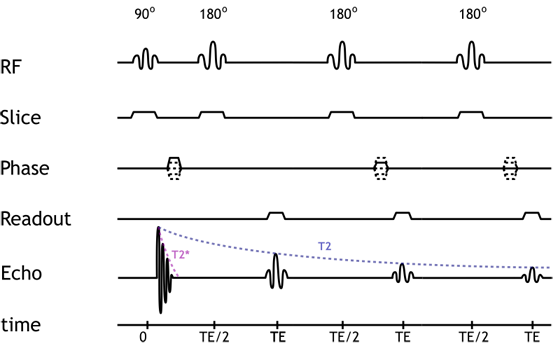
Pulse diagram of a 3-echo fast spin echo sequence. Note that the sequence only has a single 90-degree pulse but multiple (3) 180-degree pulses. Notice how the strength of each echo diminishes over time, according to the tissue T2. For each echo, a different phase-encoding gradient strength is used.
The number of echoes is referred to as the echo train length or ETL. Typical numbers might be 8-16 echoes for a FSE sequence. While the TE (echo time) is straighforward for a standard SE sequence, it is slightly more complicated for FSE. In fact, we are acquiring many echoes each with a different echo time. Thus, instead of a TE, we have an 'effective TE' that reflects the T1/T2 weighting of the sequence. Recall (or review) that multiple echoes are used to construct K-space for each slice; the peripheral echoes contribute to detail resolution, while the central echoes contribute to contrast (i.e. T1/T2 weighting). We can then understand that the effective TE reflects the time for the echo that forms the center of K-space. Note that this means that for the same effective TE, the time between the 180-degree pulse and the echo is much shorter (since we will collect several echoes before we get to the one to use for the center of K-space).
Compared with standard SE, FSE images are more T2-weighted, since even if the effective TE may be similar, many of the echoes will be acquired at much longer echo times that give more T2 weighting. Several other interesting phenomena occur with FSE images, including: (1) susceptibility decreases because of decreased time for dephasing between 180-degree pulses; (2) fat becomes bright on T2-weighted images because of loss of J-coupling. (For more advanced information on these topics, look at the excellent discussions in MRI-q on susceptibility and J-coupling.)
More recently, ultrafast FSE sequences have been developed that acquire the entire slice in one sequence - often called single-shot sequences. They typically use half-Fourier acquisition to cut in half the number of lines of K-space needed. These sequences go by names such as HASTE (Siemens) and SS-FSE (GE) and involve ETLs of 128-256. Long ETLs are limited by poor signal in the later echoes, so in order to improve signal, the 180-degree pulses are shortened, and the space between successive pulses is shortened (with high bandwidth readout). These sequences are extremely fast, acquiring a slice in under a second! The disadvantages of these sequences are: relatively lower SNR (because of high bandwidth and poor signal in the later echoes) and heavy T2 weighting.
Gradient Echo
An alternative to the spin echo-based sequences is the gradient echo sequence (GRE). This sequence does not use a 180-degree refocusing pulse and thus retains T2* dephasing. This can be an advantage if we want to accentuate susceptibility (e.g. we are looking for iron deposition); it is also much faster, since we do not have to wait for the rephasing after that pulse.
How do we form an echo without a 180 degree pulse? All MR sequences require a readout RF gradient for frequency encoding. This gradient is on during readout; recall that any gradient across the image causes dephasing of protons. This is simply because protons within even a single voxel will be precessing at slightly different frequencies because of that gradient. We can easily reverse this process by reversing the gradient for the same length of time. Ideally, we would like the peak signal to occur in the middle of the signal - thus forming an echo:
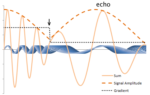
Illustration of proton rephasing in a gradient echo. The plot displays the precession of multiple protons, blue, in the presence of a gradient, black. The sum and signal amplitude are drawn in orange: the amplitude is what is detected by the MR scanner. Notice that the amplitude drops in the presence of the gradient. However, when the gradient is reversed (arrow), the dephasing reverses - the protons rephase to form an echo.
The illustration above does not include T2/T2* effects, which do occur in the GRE sequence. In fact, the presence of the readout gradient initially speeds the already-occuring T2* dephasing, which is reversed with the gradient reversal. The peak of the signal then reflects simply the T2* decay of the tissue. Because T2 effects are not negated, signal loss is much more rapid with GRE sequences, and thus much shorter TEs are typically used. (Again, we can use a shorter TE because we do not have to wait for the 180-degree pulse and rephasing.) The shorter TE allows much shorter TRs to be used, which increases T1 weighting and, more importantly, allows us to repeat the pulse sequence more quickly (to acquire more phase-encoding steps).
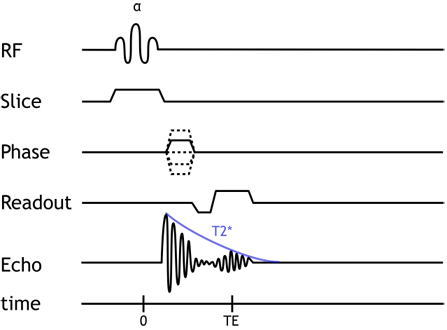
Gradient Echo pulse sequence. Notice that the echo is formed within (from) the FID. This explains why very short TEs are needed and why T2* dephasing occurs in this sequence.
Flip Angle. Most GRE sequences use an initial excitation pulse of less than 90 degrees. The so-called flip angle or α affects the amount of longitudinal magnetization that is rotated ('flipped') into the xy plane. Using a small flip angle allows a large amount of longitudinal magnetization to remain - and be available for the next repetition. This is important in GRE sequences which are typically used with very short TRs for rapid repetition. If we used up all of the longitudinal magnetization and had a short TR, not enough would recover for us to use in the next repetition. In other words, the signal (and SNR) of the sequence would be very poor. The disadvantage of small flip angles is that they decrease the T1 contrast of the sequence (for the same reason as lengthening the TR does).
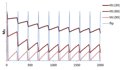
Illustration of the recovery of longitudinal magnetization in a GRE sequence with short TR and varying flip angles over successive applications of the pulse sequence. Given the short TR, there is not much time for the longitudinal magnetization (Mz, red) to recover. Using small flip angles (e.g. 30 degrees, 60 degrees) allows a larger fraction of the longitudinal magnetization to remain, so recovery is shorter. The 90 degree flip angle gives the lowest amount of signal (light red).
Spoiling. Generally when we discuss GRE sequences, we mean spoiled gradient echo sequences. Recall that the advantage of GRE is that we can use very short TR (since we do not need to wait for the 180 degree pulse and rephasing). The TRs are sufficiently short that there is some residual transverse magnetization left over at the end of each repetition. While the FID is gone, in a similar way to the 180-degree pulse causing rephasing of protons in a spin echo sequence after the FID, successive pulses (repetitions) in the GRE sequence can create spin echoes. This will alter the image contrast. Most GRE sequences do not want this, so they will employ a strong 'spoiling' or 'crushing' gradient at the end of each repetition to completely dephase the residual transverse magnetization.
Steady-State Free Precession
Instead of spoiling the residual transverse magnetization at the end of each repetition, we can keep it and use it to add to our signal. There are a number of different ways of doing this, which are termed "steady-state" MR sequences because they keep the transverse magnetization for each repetition, eventually reaching an equilibrium or steady-state of transverse magnetization. These different sequences are covered in detail in an excellent Radiographics article. Our focus here will be on the balanced (also known as fully refocused) steady-state free precession (SSFP) sequences, which are known as TrueFISP (Siemens) or FIESTA (GE). These represent the most commonly used of the SSFP sequences and have found wide application in cardiac MRI and non-contrast MR angiography, for reasons discussed below.
The balanced SSFP sequence is designed to fully compensate for all gradient dephasing from one repetition to the next. In other words, for each gradient applied, a reverse gradient is applied at the end of the sequence to reverse its effects; this is also true for the flip pulse, which alternates between positive and negative angles in successive repetitions. This approach maximizes the signal we can obtain, since we reverse gradient-based dephasing. Additionally, the balanced SSFP sequence is relatively insensitive to motion and blood flow-based dephasing, since the balanced gradients have the triphasic design that is the same used for flow compensation. Since we are using a steady-state magnetization and are refocusing our dephasing, we can repeat the sequence very quickly: the balanced SSFP sequence is extremely fast, with a TR of approximately 6 seconds.

Pulse Sequence Diagram for the balanced SSFP sequence.
Tissue contrast (T1 and T2 weighting) is complicated in SSFP sequences because of the combination of the initial excitation (FID) signal and residual transverse magentization, both of which contribute to the steady state (equilibrium magnetization). Balanced SSFP images are weighted by the ratio T2/T1. These sequences are often referred to as 'bright-blood' because blood is very bright as compared to vessel walls or myocardium; both flowing and stationary or even mildly turbulent blood retains bright signal because of the intrinsic flow compensation, as discussed above.
The fast imaging allows for cine acquisitions in cardiac MRI (i.e. making movies over the cardiac cycle). It also allows for free breathing abdominal imaging. Because SSFP is a GRE sequence, it remains sensitive to magnetic field inhomogeneities, and you will often see 'zebra' or banding artifacts, particularly at the edges of the image.
Echo Planar Imaging
The final major MR sequence category we will discuss here is echo planar imaging (EPI). This sequence is principally used in diffusion weighed imaging (DWI). The gradients used for DWI are discussed separately in the DWI article. Here we will discuss the underlying MR sequence used for most DWI. Diffusion requires extremely fast imaging because any patient motion will completely overwhelm the small molecular motions we are trying to measure.
The EPI sequence utilizes rapidly switching gradients to acquire the entirety of k-space within one spin echo. Multiple gradient echoes are formed within the single spin echo. By using varying gradient strengths, we obtain successive phase encoding steps and thereby complete the k-space matrix within that spin echo. Alternating the frequency-encoding gradient lets us 'sweep' back and forth across the frequency-encoding direction with each phase encoding step (and the alternation is what creates the gradient echoes).

Pulse Sequence Diagram for EPI. Note multiple gradient echoes formed within a spin echo. Each pulse of the phase encoding gradient begins a new line in k-space.
Echo planar imaging can be performed based on gradient echo or inversion recovery sequences, as well. Additionally, often instead of acquiring the entire k-space matrix in one shot, k-space will be 'segmented' or acquired in several chunks over the course of, say, 3-4 repetitions.
Because of the successive application of gradients, even though the base sequence is spin echo, EPI exhibits marked sensitivity to magnetic field inhomogeneities. Additionally, the successive gradients cause phase accumulation across the sequence, which results in an unusual degree of chemical shift. Chemical shift (difference between fat and water encoding) can be as much as half of the entire image.
Take-Home Points
- In the presence of a homogeneous magnetic field, protons will tend to line up along it. We can then excite (rotate) these protons into the xy-plane and, using additional pulses, capture how long it takes them to return to their initial state. Tissue contrast, discussed in detail elsewhere, is determined by how long we wait after the excitation and between successive excitations.
- The spin echo (SE) sequence uses an additional, 180-degree pulse, to flip protons and generate an echo as they rephase. This negates T2* effects from magnetic field inhomogeneity. It also provides better signal but is slower. Fast spin echo (FSE) uses many successive 180-degree pulses to speed acquisition.
- The gradient echo (GRE) sequence does not use a 180-degree pulse; dephasing occurs according to T2*, which is much more rapid. The sequence is overall much faster and allows for rapid repetition. However, it is affected by field inhomogeneity.
- Balanced steady-state free precession sequences differ from standard GRE by not spoiling (actively dephasing) residual transverse magentization. Rather, SSFP sequences preserve and reuse transverse magnetization to form a steady-state magnetization that is a combination of a spin echo and gradient echo. Balanced SSFP sequences are extremely fast and provide good signal, although tissue contrast is a mixture of T2 and T1.
- Echo planar imaging (EPI) is perhaps the fastest sequence available and is the most common sequence used for diffusion-weighted imaging. It essentially forms rapidly alternating gradient echoes within a spin echo sequence.
References
- Hanson, LG. "Is Quantum Mechanics Necessary for Understanding Magnetic Resonance?" Concepts in Magnetic Resonance Part A, Vol. 32A(5) 329340 (2008)
- Hashemi, R. H., Bradley, W. G. & Lisanti, C. J. MRI: the basics. (Lippincott Williams & Wilkins, 2010).
- MRI-q: articles on susceptibility and J-coupling in FSE.
- Chavhan GB, et al. "Steady-State MR Imaging Sequences: Physics, Classification, and Clinical Applications." Radiographics, Vol 28(4) 1147 (2008).
- Poustchi-Amin M, et al. "Principles and Applications of Echo-planar Imaging: A Review for the General Radiologist." Radiographics, Vol 21(3) 767 (2001).
Images and Content Copyright 2014 Mark Hammer. All rights reserved.